3 Exploratory and descriptive analysis with R
3.1 Working example - record sales data
Let’s import the data
Let’s look at the data
3.2 Let’s make sure our data types are correct #1
- This variable is currently stored as charcters, not as a factor / category variable
- We can save it as a factor
3.3 Measures of central tendency
The main measures of central tendency are: - Mean - Median - Mode
3.3.1 Mean
“What is the mean of album sales?”
3.3.2 Trimmed mean
- The trimmed mean is used to reduce the influence of outliers on the summary
3.3.3 Median
“What is the median amount of Airplay?”
3.3.4 Mode
“What is the most common attractiveness rating of bands?”
- The easiest way to get the mode in R is to generate a frequency table
- We can then look for the most frequently occuring response
3.4 Measures of dispresion or variance
3.4.1 Range
The range is the difference between the lowest and highest values
- You can calculate it using these values
- Or you can use the range command to get the min and max values in one go
3.4.2 Interquartile range
- We know that the median is the “middle” of the data = 50th percentile
- The interquatile range is the difference between the values at the 25th and 75th percentiles
- Interquartile range = 36 - 19.75 = 16.25
Sum of squares
- The difference between each value and the mean value, squared, and then summed together
3.4.3 Variance
- Variance: Sum of sqaures divided by n-1
3.4.4 Standard deviation
- Standard deviation is square root of the variance
- Can be calculated using the sd() command
3.5 Skewness and Kurtosis
3.5.1 Assessing skewness of distribution #1
- It is possible to use graphs to view the distribution
- We will focus on graphic presentation of data next week

3.5.2 Assessing skewness of distribution #2
- We can check raw skewness value using the skew() command in the psych package
3.5.3 Kurtosis
| informal term | technical name | kurtosis value |
|---|---|---|
| “too flat” | platykurtic | negative |
| “just pointy enough” | mesokurtic | zero |
| “too pointy” | leptokurtic | positive |
3.5.4 Assessing normality of distribution
- We can use the shapiro-wilk test of normality
- This is part of “base” r (no package needed)
3.6 Getting and overall summary
3.6.1 summary() - in “base R”
    Adverts             Sales          Airplay         Attract
 Min.   :   9.104   Min.   : 10.0   Min.   : 0.00   Min.   : 1.00
 1st Qu.: 215.918   1st Qu.:137.5   1st Qu.:19.75   1st Qu.: 6.00
 Median : 531.916   Median :200.0   Median :28.00   Median : 7.00
 Mean   : 614.412   Mean   :193.2   Mean   :27.50   Mean   : 6.77
 3rd Qu.: 911.226   3rd Qu.:250.0   3rd Qu.:36.00   3rd Qu.: 8.00
 Max.   :2271.860   Max.   :360.0   Max.   :63.00   Max.   :10.00
     Genre
 Country:46
 HipHop :53
 Metal  :48
 Pop    :53
3.6.2 describe() - in the “psych” package #1
| vars | n | mean | sd | median | trimmed | mad | min | max | range | skew | kurtosis | se | |
|---|---|---|---|---|---|---|---|---|---|---|---|---|---|
| Adverts | 1 | 200 | 614.4123 | 485.655208 | 531.916 | 560.80516 | 489.0882 | 9.104 | 2271.86 | 2262.756 | 0.8399360 | 0.1687385 | 34.3410091 |
| Sales | 2 | 200 | 193.2000 | 80.698957 | 200.000 | 192.68750 | 88.9560 | 10.000 | 360.00 | 350.000 | 0.0432729 | -0.7157339 | 5.7062779 |
| Airplay | 3 | 200 | 27.5000 | 12.269585 | 28.000 | 27.46250 | 11.8608 | 0.000 | 63.00 | 63.000 | 0.0588275 | -0.0924910 | 0.8675907 |
| Attract | 4 | 200 | 6.7700 | 1.395290 | 7.000 | 6.88125 | 1.4826 | 1.000 | 10.00 | 9.000 | -1.2668371 | 3.5555040 | 0.0986619 |
| Genre* | 5 | 200 | 2.5400 | 1.115627 | 3.000 | 2.55000 | 1.4826 | 1.000 | 4.00 | 3.000 | -0.0242500 | -1.3661364 | 0.0788867 |
3.6.3 describe() - in the “psych” package #2
- We can describe by factor variables
 Descriptive statistics by group
group: Country
        vars  n   mean     sd median trimmed    mad  min     max   range  skew
Adverts    1 46 656.22 507.96 574.14  620.40 581.96  9.1 1985.12 1976.01  0.51
Sales      2 46 201.74  73.64 210.00  200.79  66.72 60.0  360.00  300.00  0.03
Airplay    3 46  29.07  10.53  28.00   28.50  11.12  9.0   54.00   45.00  0.44
Attract    4 46   6.52   1.63   7.00    6.71   1.48  1.0   10.00    9.00 -1.49
Genre*     5 46   1.00   0.00   1.00    1.00   0.00  1.0    1.00    0.00   NaN
        kurtosis    se
Adverts    -0.65 74.89
Sales      -0.52 10.86
Airplay    -0.10  1.55
Attract     3.54  0.24
Genre*       NaN  0.00
------------------------------------------------------------
group: HipHop
        vars  n   mean     sd median trimmed    mad   min  max   range  skew
Adverts    1 53 606.32 452.84 601.43  568.33 501.36 10.65 2000 1989.35  0.70
Sales      2 53 199.62  92.71 200.00  200.70 103.78 10.00  360  350.00 -0.10
Airplay    3 53  28.09  13.86  30.00   28.33  14.83  0.00   55   55.00 -0.14
Attract    4 53   6.96   1.13   7.00    7.00   1.48  3.00    9    6.00 -0.80
Genre*     5 53   2.00   0.00   2.00    2.00   0.00  2.00    2    0.00   NaN
        kurtosis    se
Adverts     0.05 62.20
Sales      -0.91 12.74
Airplay    -0.83  1.90
Attract     2.03  0.15
Genre*       NaN  0.00
------------------------------------------------------------
group: Metal
        vars  n   mean     sd median trimmed    mad  min     max   range  skew
Adverts    1 48 693.45 534.06  593.0  640.19 521.34 45.3 2271.86 2226.56  0.92
Sales      2 48 197.71  75.18  200.0  198.25  88.96 40.0  340.00  300.00 -0.07
Airplay    3 48  27.96  11.37   27.5   28.00  11.12  2.0   57.00   55.00  0.02
Attract    4 48   6.85   1.34    7.0    6.90   1.48  2.0    9.00    7.00 -0.84
Genre*     5 48   3.00   0.00    3.0    3.00   0.00  3.0    3.00    0.00   NaN
        kurtosis    se
Adverts     0.21 77.08
Sales      -0.94 10.85
Airplay    -0.26  1.64
Attract     1.74  0.19
Genre*       NaN  0.00
------------------------------------------------------------
group: Pop
        vars  n   mean     sd median trimmed    mad   min     max   range  skew
Adverts    1 53 514.63 446.04  429.5  453.85 438.01 15.31 1789.66 1774.35  1.01
Sales      2 53 175.28  77.92  160.0  171.86  88.96 40.00  360.00  320.00  0.34
Airplay    3 53  25.13  12.75   26.0   25.02  11.86  1.00   63.00   62.00  0.25
Attract    4 53   6.72   1.47    7.0    6.81   1.48  1.00    9.00    8.00 -1.11
Genre*     5 53   4.00   0.00    4.0    4.00   0.00  4.00    4.00    0.00   NaN
        kurtosis    se
Adverts     0.27 61.27
Sales      -0.67 10.70
Airplay     0.46  1.75
Attract     2.51  0.20
Genre*       NaN  0.00
3.7 Basic statistical tests (more detail in later sections)
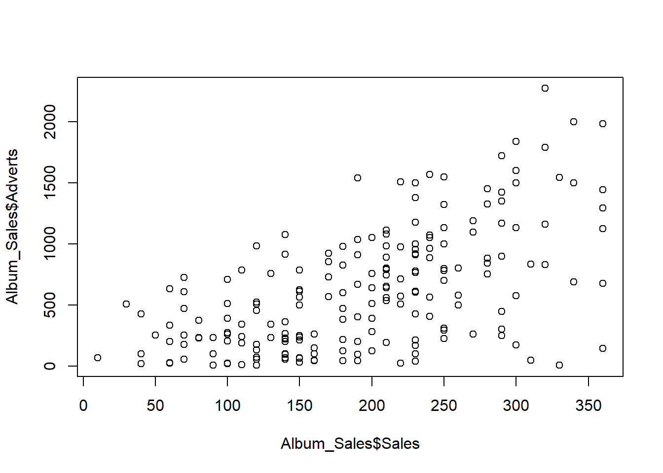
3.7.1 Corrleation
“Is there a relationship between advert spend and sales?”
- We would use an correlational analysis to answer this question
“Is there a relationship between advert spend and sales?”
- We would use an correlational analysis to answer this question
    Pearson's product-moment correlation

data:  Album_Sales$Sales and Album_Sales$Adverts
t = 9.9793, df = 198, p-value < 2.2e-16
alternative hypothesis: true correlation is not equal to 0
95 percent confidence interval:
 0.4781207 0.6639409
sample estimates:
      cor
0.5784877
3.7.2 Tests of difference - t-test
“Is there a significant difference in sales between the Country and Hip-hop musical genres?”
- We would use a t-test to answer this question
myTtestData <- Album_Sales %>% filter(Genre == c("Country", "HipHop"))

t.test(myTtestData$Sales ~ myTtestData$Genre)
    Welch Two Sample t-test

data:  myTtestData$Sales by myTtestData$Genre
t = 0.80489, df = 40.62, p-value = 0.4256
alternative hypothesis: true difference in means between group Country and group HipHop is not equal to 0
95 percent confidence interval:
 -27.80146  64.62904
sample estimates:
mean in group Country  mean in group HipHop
             216.0000              197.5862
3.7.3 Tests of difference - ANOVA
“Is there a significant difference in sales between all musical genres?”
- We would use an ANOVA to answer this question