6 Correlation in R
- Conduct and interpret a correlation analysis in R
6.1 What is Correlation?
Correlation is a measure of the strength and direction of a relationship between two variables. It is most commonly used when we want to see if there is a relationship between two continuous variables. However, it is possible to run correlations between a continuous and a categorical variable (this is known as point-biserial correlation) or between two categorical variables (this is known as phi coefficient).
Sticking to the more conventional form of correlation; when we calculate correlation, we get an r value of between -1 and 1. This tells us two things:
The closer the value is to 1, the stronger the relationship. The closer the value is to 0, the weaker the relationship.
The sign of the value tells us the direction of the relationship. Positive values indicate a positive relationship (i.e. as one variable increases, so does the other). Negative values indicate a negative relationship (i.e. as one variable increases, the other decreases).
We also often calculate the significance of the correlation, which tests against a null hypothesis that the correlation is 0. This is not part of the correlation per se, but it is often part of correlational research questions.
6.2 Visualising correlation
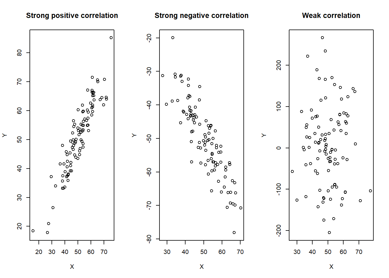
We can visualise correlation using a scatterplot. This is a graph where each data point is plotted on a graph, with one variable on the x axis and the other on the y axis. If the data points form something resembling a straight line, with all of the data points in a consistent pattern, then we have a strong correlation. If the data points are scattered, then we have a weaker correlation. However, if the data points are inconsistent or more diffuse, the correlation is weaker. The direction of the line tells us the direction of the correlation.
Visualising the data in this way can give us a good idea of the strength and direction of the correlation. However, it is not a substitute for running the correlation itself. At the same time, correlation coefficients can be misleading on their own. It is always a good idea to visualise the data as well.
6.3 How is correlation calculated?
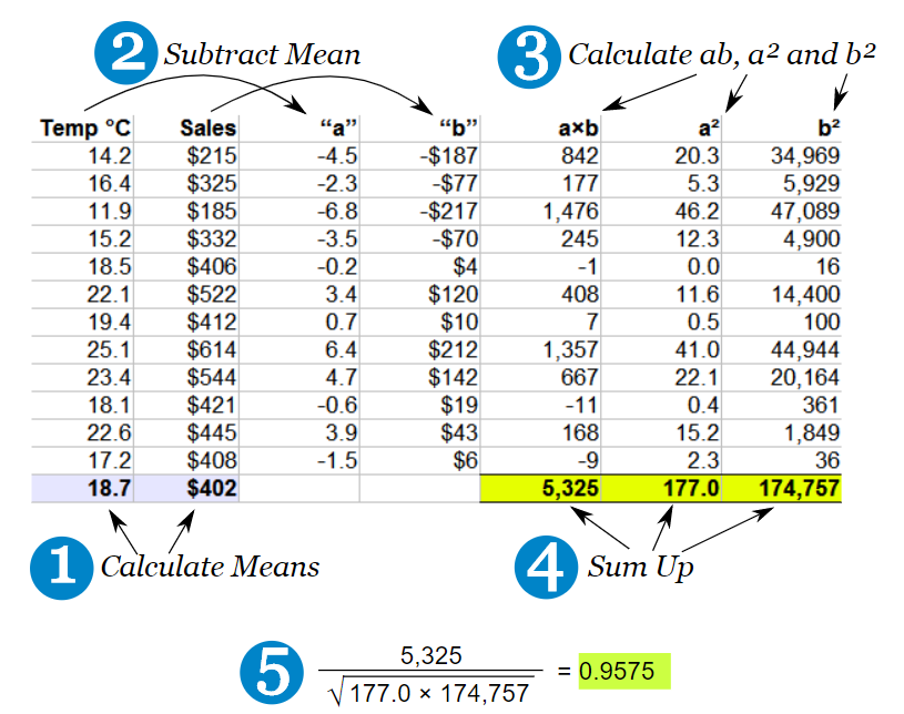
Correlation can be thought of as covariance divided by individual variance. Covariance is a measure of how much two variables change together. Variance is a measure of how much a variable changes on its own. When we divide covariance by variance, we get a value that is standardised and can be compared across different data sets.
If the changes are consistent with both variables (i.e. the covariance is higher and the individual variance is lower), then the final correlation value will be higher. However, if the changes are inconsistent (i.e. the covariance is lower and the individual variance is higher), then the final correlation value will be lower.


6.4 Which correlation to use?
When we run correlation in R, we use the cor.test() command. This command will give us the correlation value, the p value and the confidence intervals.
We can specify a Pearson correlation (the default) or a Spearman correlation (for non-parametric data).
6.4.1 Running correlation in R
- R can run correlations using the cor.test() command
cor.test(regression_data$treatment_duration,regression_data$aggression_level)
    Pearson's product-moment correlation

data:  regression_data$treatment_duration and regression_data$aggression_level
t = -9.5503, df = 98, p-value = 1.146e-15
alternative hypothesis: true correlation is not equal to 0
95 percent confidence interval:
 -0.7838251 -0.5765006
sample estimates:
       cor
-0.6942996
In the above example, we are testing the correlation between treatment duration and aggression level. Each variable is separated by a comma.
6.4.2 Interpreting the output
- The r value tells us the strength and direction of the relationship
- In the output it is labelled as “cor” (short for correlation)
Correlation values can range from -1 to 1. The closer the value is to 1, the stronger the relationship. The closer the value is to 0, the weaker the relationship. Positive values indicate a positive relationship (i.e. as one variable increases, so does the other). Negative values indicate a negative relationship (i.e. as one variable increases, the other decreases).
cor.test(regression_data$treatment_duration,regression_data$aggression_level)
    Pearson's product-moment correlation

data:  regression_data$treatment_duration and regression_data$aggression_level
t = -9.5503, df = 98, p-value = 1.146e-15
alternative hypothesis: true correlation is not equal to 0
95 percent confidence interval:
 -0.7838251 -0.5765006
sample estimates:
       cor
-0.6942996
6.4.3 Check the significance of the correlation
- We can see that the significance by looking at the p value
- The significance is 1.146^-15
- This means: 0.0000000000000001146
- Therefore p value < 0.05
cor.test(regression_data$treatment_duration,regression_data$aggression_level)
    Pearson's product-moment correlation

data:  regression_data$treatment_duration and regression_data$aggression_level
t = -9.5503, df = 98, p-value = 1.146e-15
alternative hypothesis: true correlation is not equal to 0
95 percent confidence interval:
 -0.7838251 -0.5765006
sample estimates:
       cor
-0.6942996 When we see a value like 1.146e-15, this is a shorthand way of writing a very small number. The e-15 means that we move the decimal point 15 places to the left. So 1.146e-15 is the same as 0.000000000000001146