Topic 12 Factor Analysis

## Warning: `read_table2()` was deprecated in
## readr 2.0.0.
## ℹ Please use `read_table()` instead.

## 
## ── Column specification ───────────────
## cols(
##   .default = col_double()
## )
## ℹ Use `spec()` for the full column specifications.

12.1 Overview

What is factor analysis
CFA versus PCA
Variance in factor analysis
Considertations for factor analysis
Identifying / extracting factors
Rotation
Cronbach’s alpha

12.2 Exploratory Factor analysis

Identify the relational structure between a set of variables in order to reduce them to a smaller set of factors
- The process of dimension reduction (identify new variables) or data summarisation (summarise what is already there)

12.2.1 Dimension reducton

Latent Variables: Not directly observable. Rather they are inferred from other responses
- Many psychological constructs (e.g. anxiety) are latent variables that we cannot directly measure.
- Rather, we can measure behaviours, cognitions and other variables that are related to the construct.

We might concptualise this as: “Responses to the questions are indicative of levels of underlying anxiety”

12.2.2 Data summarisation

Index Variables or Components: A weighted summary of measured variables that contribute to the component variable
“Principal components are variables of maximal variance constructed from linear combinations of the input features”

We might conceptualise this as: “We can reduce these measures/questions to a smaller set of higher order, independent, composite variables”

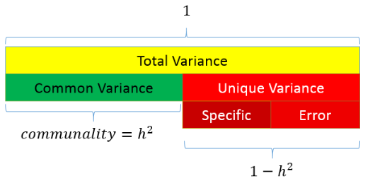
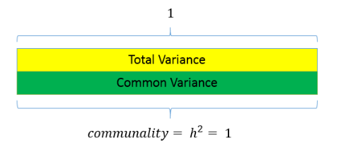
12.3 Variance in exploratory factor analysis

There are two common methods of exploratory factor analysis: Common Factor analysis and Principal Component Analysis

CFA assumes that there are two types of variance: common and unique

12.3.1 Variance in PCA

PCA only assumes common variance

12.3.2 Variance in CFA

Due to these different approaches, PCA is considered to be reflective of the current sample but not generalisable to the wider population
Whereas, CFA is considered appropriate for hypothesis testing and making inferences to the population

12.4 What is factor analysis?

If we measure several variables (or questions), we can examine the correlation between sets of these variables
- Such a correlation matrix is known as an R Matrix (r because correlation)
If there are clusters of correlations between a number of the variables (or questions), this indicates that they might be linked to the same underlying dimension (or latent variable)
The researcher should use informed judgement when assessing the appropriateness of variables for inclusion

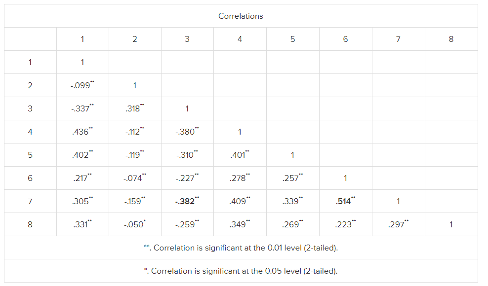An r matrix example

12.5 Considerations with factor analysis

Sample size:
- Must be more data points than variables being measured
- A common rule of thumb is at least 10 per variable
- There are tests to assess sample size adequacy (e.g. Kaiser-Meyer test should be greater than 0.5)
Inter-correlation:
- There must be sufficient correlation between the variables being measured
- A high number of correlations over 0.3
- Can be tested using Bartlett test of sphericity (sig. result means factor analysis can be used)

Other things to check (see Field, 2018)

The quality of analysis depends upon the quality of the data (GI/GO).
Avoid multicollinearity:
- several variables highly correlated, r > .80.
- Determinent: should be greater than 0.00001
Avoid singularity:
- some variables perfectly correlated, r = 1.
Screen the correlation matrix, eliminate any variables that obviously cause concern.

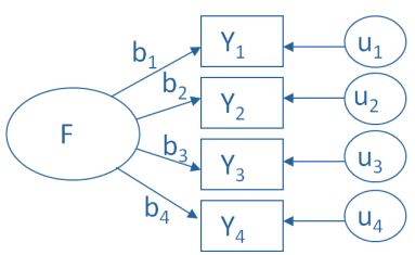
12.6 Representing factor analysis

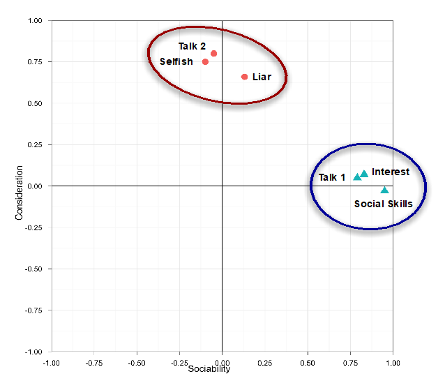
We can represent factors visually based on the strength of their inter-correlations - Here, the axis of the graph represents a factor or latent variable

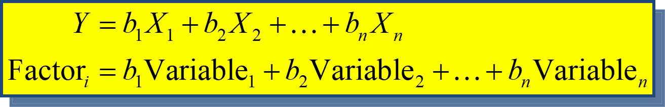
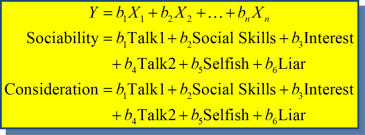
We can also represent factor analysis using a regression equation - Here the beta values represent the extent to which the variable “loads onto” a particular factor

Example: Statistics anxiety

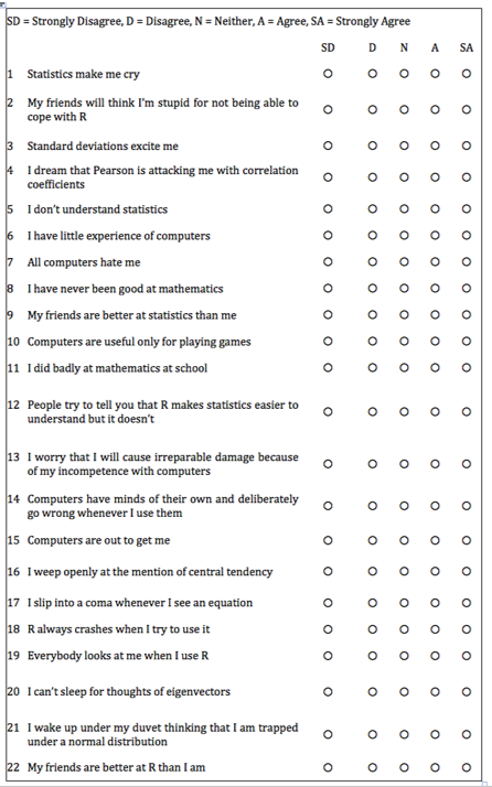
Many people get anxious about statistics
We can ask them about their experience in a number of ways (e.g. questions compiled by students in a stats class)
Their responses might indicate that stats anxiety has a number of dimensions
- i.e. it is a multi-dimensional construct, as opposed to a unitary construct

12.7 Step 1: Create a correlation matrix

raq.matrix <- cor(raq)

raq.matrix

##              Q01         Q02
## Q01  1.000000000 -0.09872403
## Q02 -0.098724032  1.00000000
## Q03 -0.336648879  0.31839020
## Q04  0.435860179 -0.11185965
## Q05  0.402439917 -0.11934658
## Q06  0.216733985 -0.07420968
## Q07  0.305365139 -0.15917448
## Q08  0.330737608 -0.04962257
## Q09 -0.092339458  0.31464054
## Q10  0.213681706 -0.08400316
## Q11  0.356786290 -0.14382984
## Q12  0.345381133 -0.19486946
## Q13  0.354646283 -0.14274026
## Q14  0.337879655 -0.16469991
## Q15  0.245752635 -0.16499581
## Q16  0.498618057 -0.16755228
## Q17  0.370550512 -0.08699527
## Q18  0.347118037 -0.16389415
## Q19 -0.189011027  0.20329748
## Q20  0.213897945 -0.20159437
## Q21  0.329153138 -0.20461730
## Q22 -0.104408664  0.23087487
## Q23 -0.004480593  0.09967828
##            Q03         Q04         Q05
## Q01 -0.3366489  0.43586018  0.40243992
## Q02  0.3183902 -0.11185965 -0.11934658
## Q03  1.0000000 -0.38046016 -0.31030879
## Q04 -0.3804602  1.00000000  0.40067225
## Q05 -0.3103088  0.40067225  1.00000000
## Q06 -0.2267405  0.27820154  0.25746014
## Q07 -0.3819533  0.40861502  0.33939179
## Q08 -0.2586342  0.34942939  0.26862697
## Q09  0.2998036 -0.12454637 -0.09570151
## Q10 -0.1933887  0.21581010  0.25820925
## Q11 -0.3506397  0.36865655  0.29782882
## Q12 -0.4099513  0.44164706  0.34674325
## Q13 -0.3179193  0.34429168  0.30182159
## Q14 -0.3707551  0.35080964  0.31533810
## Q15 -0.3123968  0.33423089  0.26137190
## Q16 -0.4186478  0.41586725  0.39491795
## Q17 -0.3273715  0.38273945  0.31041722
## Q18 -0.3752329  0.38200149  0.32209148
## Q19  0.3415737 -0.18597751 -0.16532210
## Q20 -0.3248338  0.24291796  0.19966945
## Q21 -0.4171878  0.41029317  0.33461494
## Q22  0.2036569 -0.09838349 -0.13253593
## Q23  0.1502065 -0.03381815 -0.04165684
##             Q06         Q07
## Q01  0.21673399  0.30536514
## Q02 -0.07420968 -0.15917448
## Q03 -0.22674048 -0.38195325
## Q04  0.27820154  0.40861502
## Q05  0.25746014  0.33939179
## Q06  1.00000000  0.51358048
## Q07  0.51358048  1.00000000
## Q08  0.22283175  0.29749696
## Q09 -0.11264384 -0.12829828
## Q10  0.32223023  0.28372299
## Q11  0.32807072  0.34474770
## Q12  0.31250937  0.42298591
## Q13  0.46640487  0.44211926
## Q14  0.40224407  0.44070276
## Q15  0.35989309  0.39136675
## Q16  0.24433888  0.38854534
## Q17  0.28226121  0.39074283
## Q18  0.51332164  0.50086685
## Q19 -0.16675017 -0.26912031
## Q20  0.10092489  0.22095420
## Q21  0.27233273  0.48300388
## Q22 -0.16513541 -0.16820488
## Q23 -0.06868743 -0.07029016
##             Q08         Q09
## Q01  0.33073761 -0.09233946
## Q02 -0.04962257  0.31464054
## Q03 -0.25863421  0.29980362
## Q04  0.34942939 -0.12454637
## Q05  0.26862697 -0.09570151
## Q06  0.22283175 -0.11264384
## Q07  0.29749696 -0.12829828
## Q08  1.00000000  0.01573316
## Q09  0.01573316  1.00000000
## Q10  0.15860850 -0.13418658
## Q11  0.62929768 -0.11552479
## Q12  0.25198582 -0.16739436
## Q13  0.31424716 -0.16743882
## Q14  0.28058958 -0.12150197
## Q15  0.29968600 -0.18657099
## Q16  0.32149420 -0.18886556
## Q17  0.59014022 -0.03681556
## Q18  0.27974433 -0.14957782
## Q19 -0.15947671  0.24931170
## Q20  0.17515089 -0.15864747
## Q21  0.29571756 -0.13594310
## Q22 -0.07917265  0.25684622
## Q23 -0.05023839  0.17077441
##             Q10         Q11
## Q01  0.21368171  0.35678629
## Q02 -0.08400316 -0.14382984
## Q03 -0.19338871 -0.35063969
## Q04  0.21581010  0.36865655
## Q05  0.25820925  0.29782882
## Q06  0.32223023  0.32807072
## Q07  0.28372299  0.34474770
## Q08  0.15860850  0.62929768
## Q09 -0.13418658 -0.11552479
## Q10  1.00000000  0.27143657
## Q11  0.27143657  1.00000000
## Q12  0.24582591  0.33529466
## Q13  0.30196707  0.42316548
## Q14  0.25468730  0.32532025
## Q15  0.29523438  0.36482687
## Q16  0.29058576  0.36907763
## Q17  0.21832214  0.58683495
## Q18  0.29250304  0.37341373
## Q19 -0.12723487 -0.19965203
## Q20  0.08406520  0.25533736
## Q21  0.19313633  0.34643407
## Q22 -0.13090831 -0.16198921
## Q23 -0.06191796 -0.08637256
##             Q12         Q13
## Q01  0.34538113  0.35464628
## Q02 -0.19486946 -0.14274026
## Q03 -0.40995127 -0.31791928
## Q04  0.44164706  0.34429168
## Q05  0.34674325  0.30182159
## Q06  0.31250937  0.46640487
## Q07  0.42298591  0.44211926
## Q08  0.25198582  0.31424716
## Q09 -0.16739436 -0.16743882
## Q10  0.24582591  0.30196707
## Q11  0.33529466  0.42316548
## Q12  1.00000000  0.48871303
## Q13  0.48871303  1.00000000
## Q14  0.43270398  0.44978632
## Q15  0.33179910  0.34219704
## Q16  0.40805908  0.35837775
## Q17  0.33269383  0.40837657
## Q18  0.49296482  0.53293713
## Q19 -0.26665953 -0.22697105
## Q20  0.29802585  0.20396327
## Q21  0.44063832  0.37443078
## Q22 -0.16728557 -0.19535632
## Q23 -0.04642506 -0.05298304
##             Q14         Q15
## Q01  0.33787966  0.24575263
## Q02 -0.16469991 -0.16499581
## Q03 -0.37075510 -0.31239678
## Q04  0.35080964  0.33423089
## Q05  0.31533810  0.26137190
## Q06  0.40224407  0.35989309
## Q07  0.44070276  0.39136675
## Q08  0.28058958  0.29968600
## Q09 -0.12150197 -0.18657099
## Q10  0.25468730  0.29523438
## Q11  0.32532025  0.36482687
## Q12  0.43270398  0.33179910
## Q13  0.44978632  0.34219704
## Q14  1.00000000  0.38011484
## Q15  0.38011484  1.00000000
## Q16  0.41841820  0.45427861
## Q17  0.35374183  0.37310235
## Q18  0.49830615  0.34287045
## Q19 -0.25405813 -0.20980230
## Q20  0.22592173  0.20625622
## Q21  0.39938896  0.29971557
## Q22 -0.16983754 -0.16790617
## Q23 -0.04847418 -0.06200665
##             Q16         Q17
## Q01  0.49861806  0.37055051
## Q02 -0.16755228 -0.08699527
## Q03 -0.41864780 -0.32737145
## Q04  0.41586725  0.38273945
## Q05  0.39491795  0.31041722
## Q06  0.24433888  0.28226121
## Q07  0.38854534  0.39074283
## Q08  0.32149420  0.59014022
## Q09 -0.18886556 -0.03681556
## Q10  0.29058576  0.21832214
## Q11  0.36907763  0.58683495
## Q12  0.40805908  0.33269383
## Q13  0.35837775  0.40837657
## Q14  0.41841820  0.35374183
## Q15  0.45427861  0.37310235
## Q16  1.00000000  0.40976309
## Q17  0.40976309  1.00000000
## Q18  0.42197911  0.37560681
## Q19 -0.26704702 -0.16288096
## Q20  0.26514025  0.20523013
## Q21  0.42054273  0.36349147
## Q22 -0.15579385 -0.12629066
## Q23 -0.08152195 -0.09167243
##             Q18        Q19         Q20
## Q01  0.34711804 -0.1890110  0.21389794
## Q02 -0.16389415  0.2032975 -0.20159437
## Q03 -0.37523290  0.3415737 -0.32483385
## Q04  0.38200149 -0.1859775  0.24291796
## Q05  0.32209148 -0.1653221  0.19966945
## Q06  0.51332164 -0.1667502  0.10092489
## Q07  0.50086685 -0.2691203  0.22095420
## Q08  0.27974433 -0.1594767  0.17515089
## Q09 -0.14957782  0.2493117 -0.15864747
## Q10  0.29250304 -0.1272349  0.08406520
## Q11  0.37341373 -0.1996520  0.25533736
## Q12  0.49296482 -0.2666595  0.29802585
## Q13  0.53293713 -0.2269710  0.20396327
## Q14  0.49830615 -0.2540581  0.22592173
## Q15  0.34287045 -0.2098023  0.20625622
## Q16  0.42197911 -0.2670470  0.26514025
## Q17  0.37560681 -0.1628810  0.20523013
## Q18  1.00000000 -0.2566318  0.23518040
## Q19 -0.25663183  1.0000000 -0.24859386
## Q20  0.23518040 -0.2485939  1.00000000
## Q21  0.43010427 -0.2748979  0.46770448
## Q22 -0.15982631  0.2339226 -0.09970186
## Q23 -0.08041698  0.1224344 -0.03466529
##             Q21         Q22
## Q01  0.32915314 -0.10440866
## Q02 -0.20461730  0.23087487
## Q03 -0.41718781  0.20365686
## Q04  0.41029317 -0.09838349
## Q05  0.33461494 -0.13253593
## Q06  0.27233273 -0.16513541
## Q07  0.48300388 -0.16820488
## Q08  0.29571756 -0.07917265
## Q09 -0.13594310  0.25684622
## Q10  0.19313633 -0.13090831
## Q11  0.34643407 -0.16198921
## Q12  0.44063832 -0.16728557
## Q13  0.37443078 -0.19535632
## Q14  0.39938896 -0.16983754
## Q15  0.29971557 -0.16790617
## Q16  0.42054273 -0.15579385
## Q17  0.36349147 -0.12629066
## Q18  0.43010427 -0.15982631
## Q19 -0.27489793  0.23392259
## Q20  0.46770448 -0.09970186
## Q21  1.00000000 -0.12902148
## Q22 -0.12902148  1.00000000
## Q23 -0.06766437  0.23036940
##              Q23
## Q01 -0.004480593
## Q02  0.099678285
## Q03  0.150206522
## Q04 -0.033818152
## Q05 -0.041656841
## Q06 -0.068687430
## Q07 -0.070290157
## Q08 -0.050238392
## Q09  0.170774410
## Q10 -0.061917956
## Q11 -0.086372565
## Q12 -0.046425059
## Q13 -0.052983042
## Q14 -0.048474181
## Q15 -0.062006650
## Q16 -0.081521950
## Q17 -0.091672426
## Q18 -0.080416984
## Q19  0.122434401
## Q20 -0.034665293
## Q21 -0.067664367
## Q22  0.230369402
## Q23  1.000000000

12.8 Step 2: Let’s check for Inter-correlation

library(corrplot)

## corrplot 0.92 loaded

corrplot(raq.matrix, method = "number")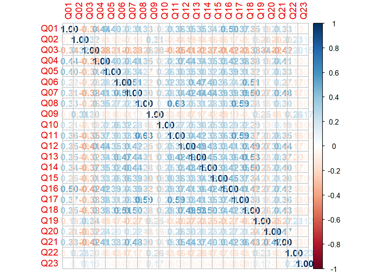

We can use bartlett’s test from the psych package

library(psych)

cortest.bartlett(raq.matrix, n=2571)

## $chisq
## [1] 19334.49
## 
## $p.value
## [1] 0
## 
## $df
## [1] 253

12.9 Step 3: Check sampling adequacy

Overall should be > 0.5

KMO(raq)

## Kaiser-Meyer-Olkin factor adequacy
## Call: KMO(r = raq)
## Overall MSA =  0.93
## MSA for each item = 
##  Q01  Q02  Q03  Q04  Q05  Q06  Q07 
## 0.93 0.87 0.95 0.96 0.96 0.89 0.94 
##  Q08  Q09  Q10  Q11  Q12  Q13  Q14 
## 0.87 0.83 0.95 0.91 0.95 0.95 0.97 
##  Q15  Q16  Q17  Q18  Q19  Q20  Q21 
## 0.94 0.93 0.93 0.95 0.94 0.89 0.93 
##  Q22  Q23 
## 0.88 0.77

12.10 Step 4: Identify number of factors

Based on Eigenvalues:
- Kaiser (1960) – retain factors with eigen values > 1.
- Joliffe (1972) – retain factors with eigen values > .70.
Use a scree plot: Cattell (1966): use ‘point of inflexion’.

12.10.1 Which rule?

Use Kaiser’s extraction when
- Less than 30 variables, communalities after extraction > 0.7
- Sample size > 250 and mean communality > 0.6
Scree plot is good if sample size is > 200

12.10.2 Scree plot

scree(raq)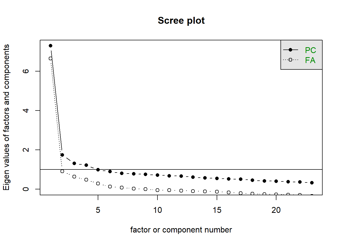

We are looking for the point of inflection
Where there is a drop-off

One approach: See how many factors we can draw a line through

12.10.3 Parallel analysis

How many dimensions of stats anxiety are captured in the questionnaire?

We can run a parallel analysis to get an indication of the number of factors contained within the data
Parallel Analysis:
- Simulates data within the same range of values as our data set
- Suggests that we retain, at maximum, the factors with eigenvalues larger than those extracted from simulated data.

library(psych)

 parallel_analysis <- fa.parallel(raq)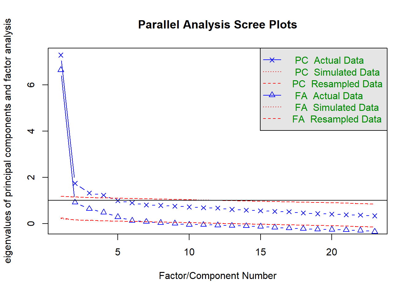

## Parallel analysis suggests that the number of factors =  6  and the number of components =  4

parallel_analysis

## Call: fa.parallel(x = raq)
## Parallel analysis suggests that the number of factors =  6  and the number of components =  4 
## 
##  Eigen Values of 
##   Original factors Resampled data
## 1             6.64           0.24
## 2             0.91           0.15
## 3             0.63           0.14
## 4             0.48           0.12
## 5             0.29           0.10
## 6             0.13           0.09
##   Simulated data Original components
## 1           0.21                7.29
## 2           0.15                1.74
## 3           0.13                1.32
## 4           0.11                1.23
## 5           0.10                0.99
## 6           0.08                0.90
##   Resampled components
## 1                 1.17
## 2                 1.15
## 3                 1.13
## 4                 1.11
## 5                 1.10
## 6                 1.08
##   Simulated components
## 1                 1.17
## 2                 1.14
## 3                 1.12
## 4                 1.11
## 5                 1.09
## 6                 1.08

12.11 Step 5: Perform factor analysis (with initial recommended # factors)

paf <- fa(raq,
nfactors = 6,
fm="pa",
max.iter = 100,
rotate = "none")

paf

## Factor Analysis using method =  pa
## Call: fa(r = raq, nfactors = 6, rotate = "none", max.iter = 100, fm = "pa")
## Standardized loadings (pattern matrix) based upon correlation matrix
##       PA1   PA2   PA3   PA4   PA5
## Q01  0.57  0.13 -0.12  0.23 -0.28
## Q02 -0.28  0.37  0.17  0.12 -0.03
## Q03 -0.60  0.25  0.20 -0.02 -0.01
## Q04  0.61  0.08 -0.06  0.18 -0.09
## Q05  0.52  0.04 -0.02  0.15 -0.17
## Q06  0.55  0.02  0.49 -0.17  0.07
## Q07  0.66 -0.03  0.22  0.03  0.11
## Q08  0.55  0.49 -0.27 -0.21  0.10
## Q09 -0.27  0.46  0.12  0.21  0.10
## Q10  0.40 -0.01  0.17 -0.09 -0.15
## Q11  0.64  0.31 -0.20 -0.27  0.08
## Q12  0.64 -0.10  0.06  0.15  0.05
## Q13  0.65  0.02  0.22 -0.06  0.06
## Q14  0.63 -0.04  0.16  0.06  0.01
## Q15  0.58 -0.01  0.07 -0.15 -0.19
## Q16  0.66 -0.02 -0.11  0.14 -0.28
## Q17  0.63  0.36 -0.15 -0.15  0.04
## Q18  0.68 -0.04  0.28  0.04  0.09
## Q19 -0.40  0.27  0.11  0.06 -0.05
## Q20  0.41 -0.17 -0.25  0.19  0.24
## Q21  0.64 -0.10 -0.11  0.27  0.28
## Q22 -0.28  0.29  0.05  0.28  0.05
## Q23 -0.13  0.18  0.08  0.23  0.01
##       PA6   h2   u2 com
## Q01 -0.19 0.52 0.48 2.3
## Q02  0.01 0.26 0.74 2.6
## Q03  0.03 0.46 0.54 1.6
## Q04 -0.03 0.42 0.58 1.3
## Q05 -0.08 0.33 0.67 1.5
## Q06 -0.01 0.57 0.43 2.2
## Q07  0.06 0.50 0.50 1.3
## Q08 -0.02 0.66 0.34 2.9
## Q09  0.03 0.35 0.65 2.4
## Q10  0.02 0.22 0.78 1.8
## Q11 -0.04 0.63 0.37 2.1
## Q12 -0.07 0.45 0.55 1.2
## Q13 -0.13 0.50 0.50 1.4
## Q14  0.01 0.42 0.58 1.2
## Q15  0.44 0.59 0.41 2.3
## Q16  0.09 0.56 0.44 1.6
## Q17  0.01 0.57 0.43 1.9
## Q18 -0.10 0.57 0.43 1.4
## Q19  0.02 0.25 0.75 2.0
## Q20  0.11 0.37 0.63 3.5
## Q21  0.10 0.60 0.40 2.0
## Q22  0.11 0.26 0.74 3.4
## Q23  0.08 0.12 0.88 3.1
## 
##                        PA1  PA2  PA3
## SS loadings           6.79 1.14 0.83
## Proportion Var        0.30 0.05 0.04
## Cumulative Var        0.30 0.34 0.38
## Proportion Explained  0.67 0.11 0.08
## Cumulative Proportion 0.67 0.78 0.86
##                        PA4  PA5  PA6
## SS loadings           0.67 0.45 0.32
## Proportion Var        0.03 0.02 0.01
## Cumulative Var        0.41 0.43 0.44
## Proportion Explained  0.07 0.04 0.03
## Cumulative Proportion 0.92 0.97 1.00
## 
## Mean item complexity =  2
## Test of the hypothesis that 6 factors are sufficient.
## 
## The degrees of freedom for the null model are  253  and the objective function was  7.55 with Chi Square of  19334.49
## The degrees of freedom for the model are 130  and the objective function was  0.23 
## 
## The root mean square of the residuals (RMSR) is  0.02 
## The df corrected root mean square of the residuals is  0.02 
## 
## The harmonic number of observations is  2571 with the empirical chi square  364.66  with prob <  3.9e-24 
## The total number of observations was  2571  with Likelihood Chi Square =  578.65  with prob <  7.6e-58 
## 
## Tucker Lewis Index of factoring reliability =  0.954
## RMSEA index =  0.037  and the 90 % confidence intervals are  0.034 0.04
## BIC =  -442.12
## Fit based upon off diagonal values = 1
## Measures of factor score adequacy             
##                                                    PA1
## Correlation of (regression) scores with factors   0.97
## Multiple R square of scores with factors          0.93
## Minimum correlation of possible factor scores     0.87
##                                                    PA2
## Correlation of (regression) scores with factors   0.83
## Multiple R square of scores with factors          0.68
## Minimum correlation of possible factor scores     0.37
##                                                    PA3
## Correlation of (regression) scores with factors   0.80
## Multiple R square of scores with factors          0.64
## Minimum correlation of possible factor scores     0.27
##                                                    PA4
## Correlation of (regression) scores with factors   0.75
## Multiple R square of scores with factors          0.56
## Minimum correlation of possible factor scores     0.12
##                                                     PA5
## Correlation of (regression) scores with factors    0.70
## Multiple R square of scores with factors           0.48
## Minimum correlation of possible factor scores     -0.03
##                                                     PA6
## Correlation of (regression) scores with factors    0.65
## Multiple R square of scores with factors           0.42
## Minimum correlation of possible factor scores     -0.17

12.11.1 Check the factor matrix

We are looking high levels of variance explained with SS loadings > 1

print(paf$loadings, cutoff=0, digits=3)

## 
## Loadings:
##     PA1    PA2    PA3    PA4    PA5   
## Q01  0.567  0.129 -0.120  0.229 -0.275
## Q02 -0.280  0.369  0.172  0.115 -0.029
## Q03 -0.603  0.245  0.199 -0.022 -0.006
## Q04  0.606  0.082 -0.056  0.184 -0.090
## Q05  0.523  0.043 -0.020  0.154 -0.167
## Q06  0.548  0.024  0.488 -0.166  0.073
## Q07  0.662 -0.026  0.223  0.030  0.107
## Q08  0.545  0.488 -0.272 -0.214  0.096
## Q09 -0.266  0.462  0.124  0.210  0.097
## Q10  0.405 -0.005  0.172 -0.090 -0.148
## Q11  0.644  0.312 -0.199 -0.270  0.085
## Q12  0.641 -0.099  0.063  0.154  0.047
## Q13  0.650  0.024  0.223 -0.058  0.061
## Q14  0.626 -0.036  0.161  0.056  0.011
## Q15  0.580 -0.007  0.072 -0.152 -0.188
## Q16  0.661 -0.016 -0.109  0.138 -0.283
## Q17  0.629  0.355 -0.155 -0.150  0.038
## Q18  0.683 -0.039  0.277  0.041  0.092
## Q19 -0.395  0.267  0.110  0.060 -0.052
## Q20  0.412 -0.171 -0.250  0.190  0.241
## Q21  0.644 -0.099 -0.110  0.270  0.283
## Q22 -0.279  0.291  0.050  0.284  0.047
## Q23 -0.130  0.182  0.081  0.235  0.011
##     PA6   
## Q01 -0.188
## Q02  0.009
## Q03  0.030
## Q04 -0.033
## Q05 -0.083
## Q06 -0.006
## Q07  0.057
## Q08 -0.020
## Q09  0.032
## Q10  0.024
## Q11 -0.037
## Q12 -0.067
## Q13 -0.134
## Q14  0.013
## Q15  0.436
## Q16  0.094
## Q17  0.006
## Q18 -0.099
## Q19  0.022
## Q20  0.114
## Q21  0.099
## Q22  0.114
## Q23  0.077
## 
##                  PA1   PA2   PA3   PA4
## SS loadings    6.786 1.140 0.827 0.667
## Proportion Var 0.295 0.050 0.036 0.029
## Cumulative Var 0.295 0.345 0.381 0.410
##                  PA5   PA6
## SS loadings    0.452 0.324
## Proportion Var 0.020 0.014
## Cumulative Var 0.429 0.443

12.11.2 Check the structure matrix

print(paf$Structure, cutoff=0, digits=3)

## 
## Loadings:
##     PA1    PA2    PA3    PA4    PA5   
## Q01  0.567  0.129 -0.120  0.229 -0.275
## Q02 -0.280  0.369  0.172  0.115 -0.029
## Q03 -0.603  0.245  0.199 -0.022 -0.006
## Q04  0.606  0.082 -0.056  0.184 -0.090
## Q05  0.523  0.043 -0.020  0.154 -0.167
## Q06  0.548  0.024  0.488 -0.166  0.073
## Q07  0.662 -0.026  0.223  0.030  0.107
## Q08  0.545  0.488 -0.272 -0.214  0.096
## Q09 -0.266  0.462  0.124  0.210  0.097
## Q10  0.405 -0.005  0.172 -0.090 -0.148
## Q11  0.644  0.312 -0.199 -0.270  0.085
## Q12  0.641 -0.099  0.063  0.154  0.047
## Q13  0.650  0.024  0.223 -0.058  0.061
## Q14  0.626 -0.036  0.161  0.056  0.011
## Q15  0.580 -0.007  0.072 -0.152 -0.188
## Q16  0.661 -0.016 -0.109  0.138 -0.283
## Q17  0.629  0.355 -0.155 -0.150  0.038
## Q18  0.683 -0.039  0.277  0.041  0.092
## Q19 -0.395  0.267  0.110  0.060 -0.052
## Q20  0.412 -0.171 -0.250  0.190  0.241
## Q21  0.644 -0.099 -0.110  0.270  0.283
## Q22 -0.279  0.291  0.050  0.284  0.047
## Q23 -0.130  0.182  0.081  0.235  0.011
##     PA6   
## Q01 -0.188
## Q02  0.009
## Q03  0.030
## Q04 -0.033
## Q05 -0.083
## Q06 -0.006
## Q07  0.057
## Q08 -0.020
## Q09  0.032
## Q10  0.024
## Q11 -0.037
## Q12 -0.067
## Q13 -0.134
## Q14  0.013
## Q15  0.436
## Q16  0.094
## Q17  0.006
## Q18 -0.099
## Q19  0.022
## Q20  0.114
## Q21  0.099
## Q22  0.114
## Q23  0.077
## 
##                  PA1   PA2   PA3   PA4
## SS loadings    6.786 1.140 0.827 0.667
## Proportion Var 0.295 0.050 0.036 0.029
## Cumulative Var 0.295 0.345 0.381 0.410
##                  PA5   PA6
## SS loadings    0.452 0.324
## Proportion Var 0.020 0.014
## Cumulative Var 0.429 0.443

12.11.3 Check eigenvalues

paf$e.values[1:6]

## [1] 7.2900471 1.7388287 1.3167515
## [4] 1.2271982 0.9878779 0.8953304

12.11.4 Check communalities

Communality for each variable: the percentage of variance that can be explained by the retained factors.
Retained factors should explain more of the variance in each variable.

paf$communality

##       Q01       Q02       Q03 
## 0.5170176 0.2585136 0.4643374 
##       Q04       Q05       Q06 
## 0.4196524 0.3341637 0.5720655 
##       Q07       Q08       Q09 
## 0.5042725 0.6649413 0.3542281 
##       Q10       Q11       Q12 
## 0.2240464 0.6328967 0.4544862 
##       Q13       Q14       Q15 
## 0.4973541 0.4223263 0.5902303 
##       Q16       Q17       Q18 
## 0.5571656 0.5700891 0.5655104 
##       Q19       Q20       Q21 
## 0.2467731 0.3686202 0.5991875 
##       Q22       Q23 
## 0.2606533 0.1178839

12.12 Step 6: Perform factor analysis (with reduced number of factors)

paf1 <- fa(raq,
nfactors = 2,
fm="pa",
max.iter = 100,
rotate = "none")

paf1

## Factor Analysis using method =  pa
## Call: fa(r = raq, nfactors = 2, rotate = "none", max.iter = 100, fm = "pa")
## Standardized loadings (pattern matrix) based upon correlation matrix
##       PA1   PA2    h2   u2 com
## Q01  0.56  0.12 0.324 0.68 1.1
## Q02 -0.28  0.39 0.228 0.77 1.8
## Q03 -0.61  0.25 0.430 0.57 1.3
## Q04  0.61  0.09 0.377 0.62 1.0
## Q05  0.52  0.05 0.276 0.72 1.0
## Q06  0.53  0.04 0.282 0.72 1.0
## Q07  0.66 -0.01 0.437 0.56 1.0
## Q08  0.53  0.40 0.445 0.56 1.9
## Q09 -0.27  0.46 0.287 0.71 1.6
## Q10  0.40  0.00 0.163 0.84 1.0
## Q11  0.63  0.27 0.472 0.53 1.3
## Q12  0.64 -0.08 0.421 0.58 1.0
## Q13  0.65  0.04 0.421 0.58 1.0
## Q14  0.63 -0.02 0.396 0.60 1.0
## Q15  0.56  0.00 0.315 0.68 1.0
## Q16  0.65 -0.01 0.428 0.57 1.0
## Q17  0.63  0.34 0.511 0.49 1.5
## Q18  0.68 -0.02 0.461 0.54 1.0
## Q19 -0.40  0.28 0.238 0.76 1.8
## Q20  0.40 -0.15 0.187 0.81 1.3
## Q21  0.63 -0.07 0.403 0.60 1.0
## Q22 -0.28  0.29 0.161 0.84 2.0
## Q23 -0.13  0.19 0.053 0.95 1.8
## 
##                        PA1  PA2
## SS loadings           6.67 1.04
## Proportion Var        0.29 0.05
## Cumulative Var        0.29 0.34
## Proportion Explained  0.86 0.14
## Cumulative Proportion 0.86 1.00
## 
## Mean item complexity =  1.3
## Test of the hypothesis that 2 factors are sufficient.
## 
## The degrees of freedom for the null model are  253  and the objective function was  7.55 with Chi Square of  19334.49
## The degrees of freedom for the model are 208  and the objective function was  1.23 
## 
## The root mean square of the residuals (RMSR) is  0.05 
## The df corrected root mean square of the residuals is  0.05 
## 
## The harmonic number of observations is  2571 with the empirical chi square  3114.53  with prob <  0 
## The total number of observations was  2571  with Likelihood Chi Square =  3155.34  with prob <  0 
## 
## Tucker Lewis Index of factoring reliability =  0.812
## RMSEA index =  0.074  and the 90 % confidence intervals are  0.072 0.077
## BIC =  1522.12
## Fit based upon off diagonal values = 0.97
## Measures of factor score adequacy             
##                                                    PA1
## Correlation of (regression) scores with factors   0.96
## Multiple R square of scores with factors          0.92
## Minimum correlation of possible factor scores     0.83
##                                                    PA2
## Correlation of (regression) scores with factors   0.78
## Multiple R square of scores with factors          0.61
## Minimum correlation of possible factor scores     0.23

plot(paf1)

12.13 Factor analysis rotation

What is rotation?

It is possible that variables load “highly” onto one factor and “medium” onto another
By rotating the factor axes, the variables are aligned with the factors that they load onto most
This helps us discriminate between factors

There are different methods of rotation

Orthogonal rotation: Assumes that factors are unrelated and keeps them that way
Oblique rotation: Assumes that factors might be related and allows them to be correlated after rotation

Are factors related? -Theoretical: Do we have logical reason for thinking they could be connected? -Based on data: Does the factor plot suggest independence or relatedness?

12.14 Step 7: Rotation

Perform factor analysis (with rotation)

paf2 <- fa(raq,
nfactors = 2,
fm="pa",
max.iter = 100,
rotate = "oblimin")

## Loading required namespace: GPArotation

## Warning in fac(r = r, nfactors =
## nfactors, n.obs = n.obs, rotate =
## rotate, : I am sorry, to do these
## rotations requires the GPArotation
## package to be installed

paf2

## Factor Analysis using method =  pa
## Call: fa(r = raq, nfactors = 2, rotate = "oblimin", max.iter = 100, 
##     fm = "pa")
## Standardized loadings (pattern matrix) based upon correlation matrix
##       PA1   PA2    h2   u2 com
## Q01  0.56  0.12 0.324 0.68 1.1
## Q02 -0.28  0.39 0.228 0.77 1.8
## Q03 -0.61  0.25 0.430 0.57 1.3
## Q04  0.61  0.09 0.377 0.62 1.0
## Q05  0.52  0.05 0.276 0.72 1.0
## Q06  0.53  0.04 0.282 0.72 1.0
## Q07  0.66 -0.01 0.437 0.56 1.0
## Q08  0.53  0.40 0.445 0.56 1.9
## Q09 -0.27  0.46 0.287 0.71 1.6
## Q10  0.40  0.00 0.163 0.84 1.0
## Q11  0.63  0.27 0.472 0.53 1.3
## Q12  0.64 -0.08 0.421 0.58 1.0
## Q13  0.65  0.04 0.421 0.58 1.0
## Q14  0.63 -0.02 0.396 0.60 1.0
## Q15  0.56  0.00 0.315 0.68 1.0
## Q16  0.65 -0.01 0.428 0.57 1.0
## Q17  0.63  0.34 0.511 0.49 1.5
## Q18  0.68 -0.02 0.461 0.54 1.0
## Q19 -0.40  0.28 0.238 0.76 1.8
## Q20  0.40 -0.15 0.187 0.81 1.3
## Q21  0.63 -0.07 0.403 0.60 1.0
## Q22 -0.28  0.29 0.161 0.84 2.0
## Q23 -0.13  0.19 0.053 0.95 1.8
## 
##                        PA1  PA2
## SS loadings           6.67 1.04
## Proportion Var        0.29 0.05
## Cumulative Var        0.29 0.34
## Proportion Explained  0.86 0.14
## Cumulative Proportion 0.86 1.00
## 
## Mean item complexity =  1.3
## Test of the hypothesis that 2 factors are sufficient.
## 
## The degrees of freedom for the null model are  253  and the objective function was  7.55 with Chi Square of  19334.49
## The degrees of freedom for the model are 208  and the objective function was  1.23 
## 
## The root mean square of the residuals (RMSR) is  0.05 
## The df corrected root mean square of the residuals is  0.05 
## 
## The harmonic number of observations is  2571 with the empirical chi square  3114.53  with prob <  0 
## The total number of observations was  2571  with Likelihood Chi Square =  3155.34  with prob <  0 
## 
## Tucker Lewis Index of factoring reliability =  0.812
## RMSEA index =  0.074  and the 90 % confidence intervals are  0.072 0.077
## BIC =  1522.12
## Fit based upon off diagonal values = 0.97
## Measures of factor score adequacy             
##                                                    PA1
## Correlation of (regression) scores with factors   0.96
## Multiple R square of scores with factors          0.92
## Minimum correlation of possible factor scores     0.83
##                                                    PA2
## Correlation of (regression) scores with factors   0.78
## Multiple R square of scores with factors          0.61
## Minimum correlation of possible factor scores     0.23

plot(paf1)

plot(paf2)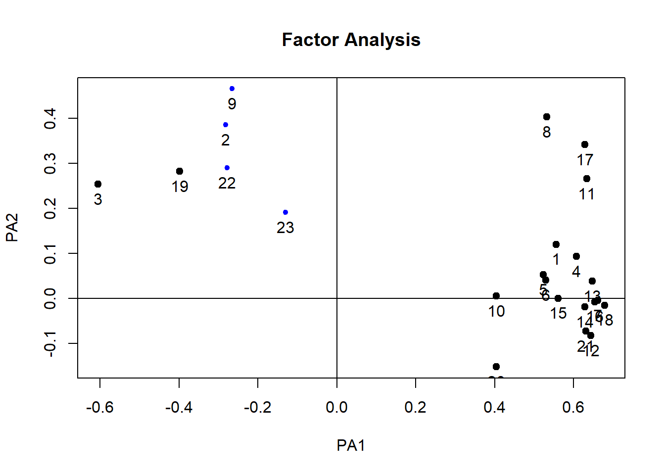

12.15 Reliability / internal consistency

12.15.1 Cronbach’s Alpha

An expansion of the split-half reliability concept
Alpha takes all possible combination of items and assesses their relationship to each other
High values above 0.7 suggest internal consistency among items

12.15.2 Chronbach’s Alpha in R

We can use the alpha() function in the psych package

library(psych)

alpha(raq)

## Warning in alpha(raq): Some items were negatively correlated with the total scale and probably 
## should be reversed.  
## To do this, run the function again with the 'check.keys=TRUE' option

## Some items ( Q02 Q03 Q09 Q19 Q22 Q23 ) were negatively correlated with the total scale and 
## probably should be reversed.  
## To do this, run the function again with the 'check.keys=TRUE' option

## 
## Reliability analysis   
## Call: alpha(x = raq)
## 
##   raw_alpha std.alpha G6(smc) average_r
##       0.75      0.77    0.83      0.13
##  S/N    ase mean   sd median_r
##  3.4 0.0065  3.3 0.39     0.23
## 
##     95% confidence boundaries 
##          lower alpha upper
## Feldt     0.74  0.75  0.77
## Duhachek  0.74  0.75  0.77
## 
##  Reliability if an item is dropped:
##     raw_alpha std.alpha G6(smc)
## Q01      0.73      0.76    0.82
## Q02      0.77      0.79    0.84
## Q03      0.79      0.81    0.85
## Q04      0.73      0.75    0.82
## Q05      0.74      0.76    0.82
## Q06      0.73      0.76    0.82
## Q07      0.73      0.75    0.82
## Q08      0.73      0.76    0.82
## Q09      0.78      0.79    0.84
## Q10      0.74      0.76    0.83
## Q11      0.73      0.75    0.81
## Q12      0.73      0.75    0.82
## Q13      0.73      0.75    0.82
## Q14      0.73      0.75    0.82
## Q15      0.73      0.76    0.82
## Q16      0.73      0.75    0.82
## Q17      0.73      0.75    0.81
## Q18      0.72      0.75    0.81
## Q19      0.78      0.80    0.85
## Q20      0.75      0.77    0.83
## Q21      0.73      0.75    0.82
## Q22      0.77      0.79    0.84
## Q23      0.77      0.79    0.84
##     average_r S/N alpha se var.r med.r
## Q01      0.12 3.1   0.0071 0.071  0.23
## Q02      0.15 3.8   0.0061 0.071  0.25
## Q03      0.16 4.2   0.0055 0.059  0.25
## Q04      0.12 3.0   0.0072 0.070  0.22
## Q05      0.12 3.1   0.0071 0.072  0.22
## Q06      0.12 3.1   0.0072 0.072  0.23
## Q07      0.12 3.0   0.0074 0.069  0.22
## Q08      0.12 3.1   0.0071 0.072  0.23
## Q09      0.15 3.8   0.0058 0.071  0.25
## Q10      0.13 3.3   0.0068 0.074  0.23
## Q11      0.12 3.0   0.0072 0.069  0.22
## Q12      0.12 3.1   0.0072 0.069  0.22
## Q13      0.12 3.0   0.0073 0.069  0.22
## Q14      0.12 3.1   0.0072 0.070  0.22
## Q15      0.12 3.1   0.0071 0.071  0.22
## Q16      0.12 3.0   0.0072 0.069  0.22
## Q17      0.12 3.0   0.0072 0.070  0.22
## Q18      0.12 3.0   0.0074 0.068  0.22
## Q19      0.15 4.0   0.0057 0.067  0.26
## Q20      0.13 3.3   0.0067 0.073  0.25
## Q21      0.12 3.1   0.0072 0.069  0.22
## Q22      0.15 3.8   0.0059 0.071  0.26
## Q23      0.14 3.7   0.0061 0.074  0.26
## 
##  Item statistics 
##        n   raw.r  std.r  r.cor r.drop
## Q01 2571  0.5598  0.581  0.564  0.492
## Q02 2571 -0.0116 -0.018 -0.114 -0.105
## Q03 2571 -0.3356 -0.361 -0.465 -0.435
## Q04 2571  0.6064  0.618  0.606  0.533
## Q05 2571  0.5365  0.546  0.516  0.454
## Q06 2571  0.5709  0.560  0.547  0.478
## Q07 2571  0.6409  0.636  0.635  0.560
## Q08 2571  0.5646  0.582  0.578  0.493
## Q09 2571  0.0587  0.020 -0.068 -0.081
## Q10 2571  0.4300  0.442  0.391  0.346
## Q11 2571  0.6078  0.628  0.633  0.540
## Q12 2571  0.5909  0.602  0.593  0.519
## Q13 2571  0.6288  0.637  0.634  0.559
## Q14 2571  0.6056  0.609  0.596  0.528
## Q15 2571  0.5433  0.550  0.526  0.457
## Q16 2571  0.5965  0.615  0.612  0.525
## Q17 2571  0.6329  0.650  0.653  0.568
## Q18 2571  0.6534  0.653  0.656  0.578
## Q19 2571 -0.1316 -0.157 -0.264 -0.248
## Q20 2571  0.3705  0.375  0.326  0.265
## Q21 2571  0.5922  0.598  0.591  0.514
## Q22 2571 -0.0063 -0.027 -0.127 -0.121
## Q23 2571  0.1030  0.084 -0.014 -0.013
##     mean   sd
## Q01  3.6 0.83
## Q02  4.4 0.85
## Q03  3.4 1.08
## Q04  3.2 0.95
## Q05  3.3 0.96
## Q06  3.8 1.12
## Q07  3.1 1.10
## Q08  3.8 0.87
## Q09  3.2 1.26
## Q10  3.7 0.88
## Q11  3.7 0.88
## Q12  2.8 0.92
## Q13  3.6 0.95
## Q14  3.1 1.00
## Q15  3.2 1.01
## Q16  3.1 0.92
## Q17  3.5 0.88
## Q18  3.4 1.05
## Q19  3.7 1.10
## Q20  2.4 1.04
## Q21  2.8 0.98
## Q22  3.1 1.04
## Q23  2.6 1.04
## 
## Non missing response frequency for each item
##        1    2    3    4    5 miss
## Q01 0.02 0.07 0.29 0.52 0.11    0
## Q02 0.01 0.04 0.08 0.31 0.56    0
## Q03 0.03 0.17 0.34 0.26 0.19    0
## Q04 0.05 0.17 0.36 0.37 0.05    0
## Q05 0.04 0.18 0.29 0.43 0.06    0
## Q06 0.06 0.10 0.13 0.44 0.27    0
## Q07 0.09 0.24 0.26 0.34 0.07    0
## Q08 0.03 0.06 0.19 0.58 0.15    0
## Q09 0.08 0.28 0.23 0.20 0.20    0
## Q10 0.02 0.10 0.18 0.57 0.14    0
## Q11 0.02 0.06 0.22 0.53 0.16    0
## Q12 0.09 0.23 0.46 0.20 0.02    0
## Q13 0.03 0.12 0.25 0.48 0.12    0
## Q14 0.07 0.18 0.38 0.31 0.06    0
## Q15 0.06 0.18 0.30 0.39 0.07    0
## Q16 0.06 0.16 0.42 0.33 0.04    0
## Q17 0.03 0.10 0.27 0.52 0.08    0
## Q18 0.06 0.12 0.31 0.37 0.14    0
## Q19 0.02 0.15 0.22 0.33 0.29    0
## Q20 0.22 0.37 0.25 0.15 0.02    0
## Q21 0.09 0.29 0.34 0.26 0.02    0
## Q22 0.05 0.26 0.34 0.26 0.10    0
## Q23 0.12 0.42 0.27 0.12 0.06    0

Here we get a warning that some of the items are negatively correlated and we should probably reverse them.
The decision to do so should be based on the logic of the questions themselves - check first
However, since cronbach’s alpha is designed to check internal consistency related to a single construct, we would expect that negative correlations would only result from:
- Items that are designed to be reverse-scored
- Questions that are related to another factor or construct
Let’s check the questionnaire
- (Q02, Q03, Q09, Q19, Q22, Q23):

It is possible to run the analysis with automatic reversal of negatively-correlated items

alpha(raq, check.keys=TRUE)

## Warning in alpha(raq, check.keys = TRUE): Some items were negatively correlated with total scale and were automatically reversed.
##  This is indicated by a negative sign for the variable name.

## 
## Reliability analysis   
## Call: alpha(x = raq, check.keys = TRUE)
## 
##   raw_alpha std.alpha G6(smc) average_r
##       0.89      0.89    0.91      0.27
##  S/N    ase mean   sd median_r
##  8.3 0.0031  3.1 0.54     0.27
## 
##     95% confidence boundaries 
##          lower alpha upper
## Feldt     0.88  0.89   0.9
## Duhachek  0.88  0.89   0.9
## 
##  Reliability if an item is dropped:
##      raw_alpha std.alpha G6(smc)
## Q01       0.88      0.89    0.90
## Q02-      0.89      0.89    0.91
## Q03-      0.88      0.89    0.90
## Q04       0.88      0.89    0.90
## Q05       0.89      0.89    0.90
## Q06       0.88      0.89    0.90
## Q07       0.88      0.89    0.90
## Q08       0.89      0.89    0.90
## Q09-      0.89      0.89    0.91
## Q10       0.89      0.89    0.90
## Q11       0.88      0.89    0.90
## Q12       0.88      0.89    0.90
## Q13       0.88      0.89    0.90
## Q14       0.88      0.89    0.90
## Q15       0.88      0.89    0.90
## Q16       0.88      0.89    0.90
## Q17       0.88      0.89    0.90
## Q18       0.88      0.88    0.90
## Q19-      0.89      0.89    0.90
## Q20       0.89      0.89    0.90
## Q21       0.88      0.89    0.90
## Q22-      0.89      0.89    0.91
## Q23-      0.89      0.90    0.91
##      average_r S/N alpha se var.r
## Q01       0.26 7.9   0.0032 0.016
## Q02-      0.28 8.4   0.0031 0.016
## Q03-      0.26 7.8   0.0033 0.017
## Q04       0.26 7.8   0.0033 0.016
## Q05       0.27 8.0   0.0032 0.017
## Q06       0.27 8.0   0.0032 0.016
## Q07       0.26 7.7   0.0034 0.016
## Q08       0.27 8.0   0.0032 0.016
## Q09-      0.28 8.4   0.0030 0.016
## Q10       0.27 8.2   0.0032 0.017
## Q11       0.26 7.8   0.0033 0.016
## Q12       0.26 7.7   0.0033 0.016
## Q13       0.26 7.7   0.0033 0.016
## Q14       0.26 7.8   0.0033 0.016
## Q15       0.26 7.9   0.0033 0.017
## Q16       0.26 7.7   0.0033 0.016
## Q17       0.26 7.8   0.0033 0.016
## Q18       0.26 7.7   0.0034 0.016
## Q19-      0.27 8.2   0.0032 0.017
## Q20       0.27 8.2   0.0032 0.017
## Q21       0.26 7.7   0.0033 0.016
## Q22-      0.28 8.4   0.0031 0.016
## Q23-      0.28 8.7   0.0030 0.014
##      med.r
## Q01   0.27
## Q02-  0.28
## Q03-  0.26
## Q04   0.26
## Q05   0.27
## Q06   0.27
## Q07   0.26
## Q08   0.27
## Q09-  0.28
## Q10   0.28
## Q11   0.26
## Q12   0.26
## Q13   0.26
## Q14   0.26
## Q15   0.27
## Q16   0.26
## Q17   0.26
## Q18   0.26
## Q19-  0.29
## Q20   0.28
## Q21   0.26
## Q22-  0.29
## Q23-  0.29
## 
##  Item statistics 
##         n raw.r std.r r.cor r.drop
## Q01  2571  0.55  0.57  0.54   0.50
## Q02- 2571  0.36  0.36  0.31   0.30
## Q03- 2571  0.65  0.64  0.62   0.59
## Q04  2571  0.61  0.61  0.59   0.55
## Q05  2571  0.54  0.55  0.52   0.48
## Q06  2571  0.56  0.55  0.53   0.49
## Q07  2571  0.67  0.67  0.65   0.62
## Q08  2571  0.51  0.53  0.51   0.46
## Q09- 2571  0.37  0.35  0.30   0.28
## Q10  2571  0.44  0.45  0.40   0.38
## Q11  2571  0.63  0.64  0.63   0.58
## Q12  2571  0.65  0.65  0.64   0.60
## Q13  2571  0.65  0.65  0.64   0.60
## Q14  2571  0.64  0.64  0.62   0.59
## Q15  2571  0.59  0.59  0.56   0.53
## Q16  2571  0.66  0.67  0.65   0.61
## Q17  2571  0.61  0.62  0.61   0.56
## Q18  2571  0.68  0.68  0.67   0.63
## Q19- 2571  0.47  0.46  0.42   0.40
## Q20  2571  0.45  0.45  0.41   0.38
## Q21  2571  0.64  0.64  0.63   0.59
## Q22- 2571  0.37  0.36  0.31   0.30
## Q23- 2571  0.23  0.22  0.15   0.15
##      mean   sd
## Q01   3.6 0.83
## Q02-  1.6 0.85
## Q03-  2.6 1.08
## Q04   3.2 0.95
## Q05   3.3 0.96
## Q06   3.8 1.12
## Q07   3.1 1.10
## Q08   3.8 0.87
## Q09-  2.8 1.26
## Q10   3.7 0.88
## Q11   3.7 0.88
## Q12   2.8 0.92
## Q13   3.6 0.95
## Q14   3.1 1.00
## Q15   3.2 1.01
## Q16   3.1 0.92
## Q17   3.5 0.88
## Q18   3.4 1.05
## Q19-  2.3 1.10
## Q20   2.4 1.04
## Q21   2.8 0.98
## Q22-  2.9 1.04
## Q23-  3.4 1.04
## 
## Non missing response frequency for each item
##        1    2    3    4    5 miss
## Q01 0.02 0.07 0.29 0.52 0.11    0
## Q02 0.01 0.04 0.08 0.31 0.56    0
## Q03 0.03 0.17 0.34 0.26 0.19    0
## Q04 0.05 0.17 0.36 0.37 0.05    0
## Q05 0.04 0.18 0.29 0.43 0.06    0
## Q06 0.06 0.10 0.13 0.44 0.27    0
## Q07 0.09 0.24 0.26 0.34 0.07    0
## Q08 0.03 0.06 0.19 0.58 0.15    0
## Q09 0.08 0.28 0.23 0.20 0.20    0
## Q10 0.02 0.10 0.18 0.57 0.14    0
## Q11 0.02 0.06 0.22 0.53 0.16    0
## Q12 0.09 0.23 0.46 0.20 0.02    0
## Q13 0.03 0.12 0.25 0.48 0.12    0
## Q14 0.07 0.18 0.38 0.31 0.06    0
## Q15 0.06 0.18 0.30 0.39 0.07    0
## Q16 0.06 0.16 0.42 0.33 0.04    0
## Q17 0.03 0.10 0.27 0.52 0.08    0
## Q18 0.06 0.12 0.31 0.37 0.14    0
## Q19 0.02 0.15 0.22 0.33 0.29    0
## Q20 0.22 0.37 0.25 0.15 0.02    0
## Q21 0.09 0.29 0.34 0.26 0.02    0
## Q22 0.05 0.26 0.34 0.26 0.10    0
## Q23 0.12 0.42 0.27 0.12 0.06    0