Topic 4 Working with data in R
4.1 By the end of this section, you will be able to:
- Import data into R from excel, SPSS and csv files
- Save data to objects
- Identify different data structures and variable types
- Convert variables from one type to another
- Order, filter and group data
- Summarise data
- Create new variables from data
4.2 In this section, we will use the Tidyverse set of packages
- A ‘toolkit’ of packages that are very useful for organsing and manipulating data
- We will use the haven package to import SPSS files
- We will use the dplyr to organise data
- Also includes the ggplot2 and tidyR packages which we will use later
To install:
install.packages(“tidyverse”)(See the previous section on installing packages)
4.3 Import data into R from excel, SPSS and csv files
We can import data from a range of sources using the Import Dataset button in the Environment tab:
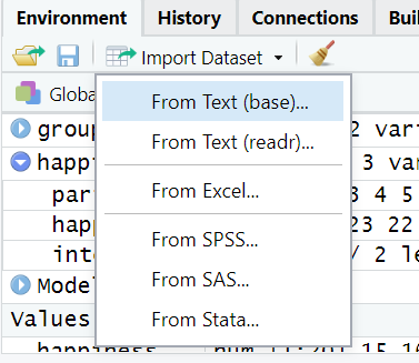
Importing data
It is also possible to import data using code, for example:
 # importing a .csv file

    library(readr)
    studentData <- read_csv("Datasets/studentData.csv")

    #importing an SPSS file

    library(haven)
    mySPSSData <- read_sav("Datasets/salesData.sav")
Once the data are imported, it will be visible in the environment:
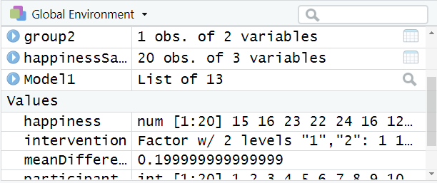
Imported data in the environment
4.5 Understanding objects in R
In R, an object is anything that is saved to memory. For example, we might do some analysis:
mean(happiness)However, in the example above, the result would appear in the console but not be saved anywhere. To store the result for reuse later, we save it to an object:
happinessMean <- mean(happiness)In the above code (reading left to right):
- We name the object “happinessMean”. This name can be anything we want.
- The arrow means that the result of the code on the right will be saved to the object on the left.
- The code on the right of the arrow calculates the mean of happiness data
When this code is run, happinessMean will be stored in the environment window:
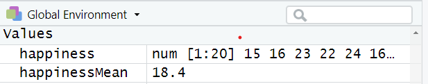
Result of a calculation in the environment
To recall an object from the environment, we can simply type its name. For example:
happinessMean## [1] 9.806722Its important to note that anything can be stored as an object in R and recalled later. This includes, dataframes, the results of statistical calculations, plots etc.
4.6 Identify different data structures and variable types
4.6.1 Data structures
There are many different types of data that R can work with. The most common type of data for most people tends to be a dataframe. A dataframe is what you might consider a “normal” 2-dimensional dataset, with rows of data and columns of variables:
A dataframe example
R can also use other data types.
A vector is a one-dimensional set of values:
# a vector example

scores <- c(1,4,6,8,3,4,6,7)
A matrix is a multi-dimensional set of values. The below example is a 3-dimensional matrix, there are 2 groups of 2 rows and 3 columns:
## , , 1
##
##      [,1] [,2] [,3]
## [1,]    1    3    5
## [2,]    2    4    6
##
## , , 2
##
##      [,1] [,2] [,3]
## [1,]    7    9   11
## [2,]    8   10   12
We will primarily work with dataframes (and sometimes vectors), as this is how the data in psychology research is usually structured.
4.6.2 Variable types
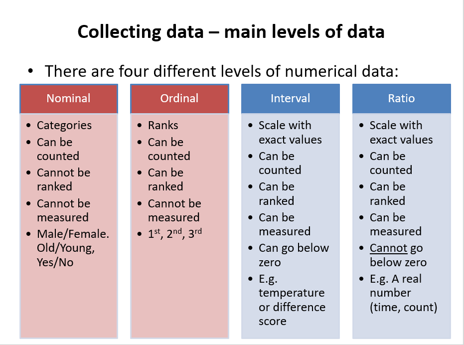
With numerical data, there are 4 key data types:
- Nominal (a category, group or factor)
- Ordinal (a ranking)
- Interval (scale data that can include negative values)
- Ratio (scale data that cannot include negative values)
 R can use all of these variable types:
- Nominal variables are called factors
- Ordinal variables are called ordered factors
- Interval and ratio variables are called numeric data and can sometimes be called integers (if they are only whole numbers) or doubles (if they all have decimal points)
R can also use other data types such as text (character) data.
4.6.3 Convert variables from one type to another
When we first import data into R, it might not recognise the data types correctly. For example, in the below data, we can see the intervention variable :
##    participant intervention happiness
## 1            1            2  6.356732
## 2            5            1  7.573209
## 3           11            1  7.864465
## 4            7            2  8.184482
## 5           16            1  8.743895
## 6            8            1  8.796175
## 7           13            1  8.883210
## 8           14            2  9.140150
## 9            9            1  9.457734
## 10          18            2  9.701410
In the intervention variable, the numbers 1 and 2 refer to different intervention groups. Therefore, the variable is a factor variable. To ensure that R understands this, we can resave the intervention variable as a factor using the as.factor() function:
happinessSample$intervention <- as.factor(happinessSample$intervention)4.7 Working with dataframes
Dataframes are the more standard data format that were are used to (think of how a dataset looks in SPSS or Excel).
In a dataframe, variables are columns and each row usually reperesents one measurement or one participant.
4.7.1 View dataframe
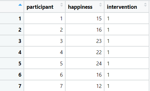
To view a dataframe, we can click on it in the environment window and it will display:
Clicking on datasets in hte environment will open them up for viewing
Viewing a dataframe
4.7.2 Refer to variables (columns) in a dataframe
Columns in a dataframe are accessed using the “$” sign. For example, to access the happiness column in the happinessSample dataframe, we would type:
happinessSample$happiness## [1] 6.356732 10.333654 12.079165
## [4] 10.474317 7.573209 12.160813
## [7] 8.184482 8.796175 9.457734
## [10] 12.181166 7.864465 11.692345
## [13] 8.883210 9.140150 9.762894
## [16] 8.743895 11.577399 9.701410
## [19] 11.387111 9.784113As we can see above, the result is then displayed.
4.8 Order, filter and group data
If you have the tidyverse package loaded, it is easy to organise and filter data.
arrange(happinessSample, happiness)## participant intervention happiness
## 1 1 2 6.356732
## 2 5 1 7.573209
## 3 11 1 7.864465
## 4 7 2 8.184482
## 5 16 1 8.743895
## 6 8 1 8.796175
## 7 13 1 8.883210
## 8 14 2 9.140150
## 9 9 1 9.457734
## 10 18 2 9.701410
## 11 15 2 9.762894
## 12 20 1 9.784113
## 13 2 1 10.333654
## 14 4 2 10.474317
## 15 19 2 11.387111
## 16 17 1 11.577399
## 17 12 2 11.692345
## 18 3 1 12.079165
## 19 6 2 12.160813
## 20 10 1 12.181166arrange(happinessSample, desc(happiness)) # Arrange in descending order## participant intervention happiness
## 1 10 1 12.181166
## 2 6 2 12.160813
## 3 3 1 12.079165
## 4 12 2 11.692345
## 5 17 1 11.577399
## 6 19 2 11.387111
## 7 4 2 10.474317
## 8 2 1 10.333654
## 9 20 1 9.784113
## 10 15 2 9.762894
## 11 18 2 9.701410
## 12 9 1 9.457734
## 13 14 2 9.140150
## 14 13 1 8.883210
## 15 8 1 8.796175
## 16 16 1 8.743895
## 17 7 2 8.184482
## 18 11 1 7.864465
## 19 5 1 7.573209
## 20 1 2 6.356732- Show clients with a happiness score of less than 4
filter(happinessSample, happiness < 4)## [1] participant intervention
## [3] happiness
## <0 rows> (or 0-length row.names)- Show Intervention group 2 with happiness scores above 7
filter(happinessSample, happiness > 7 & intervention == 2)## participant intervention happiness
## 1 4 2 10.474317
## 2 6 2 12.160813
## 3 7 2 8.184482
## 4 12 2 11.692345
## 5 14 2 9.140150
## 6 15 2 9.762894
## 7 18 2 9.701410
## 8 19 2 11.387111- Group by intervention and show the mean happiness score
happinessSample %>% group_by(intervention) %>% summarise(mean = mean(happiness))## # A tibble: 2 × 2
## intervention mean
## <fct> <dbl>
## 1 1 9.75
## 2 2 9.874.9 Create new variables from data
To create new variables from data, we can use the mutate() function.
For example, let’s say we wanted to calculate the difference between each person’s happiness score and the mean happiness score.
We could do the following:
happinessSample %>% mutate(difference = happiness - mean(happiness))## participant intervention happiness
## 1 1 2 6.356732
## 2 2 1 10.333654
## 3 3 1 12.079165
## 4 4 2 10.474317
## 5 5 1 7.573209
## 6 6 2 12.160813
## 7 7 2 8.184482
## 8 8 1 8.796175
## 9 9 1 9.457734
## 10 10 1 12.181166
## 11 11 1 7.864465
## 12 12 2 11.692345
## 13 13 1 8.883210
## 14 14 2 9.140150
## 15 15 2 9.762894
## 16 16 1 8.743895
## 17 17 1 11.577399
## 18 18 2 9.701410
## 19 19 2 11.387111
## 20 20 1 9.784113
## difference
## 1 -3.44999023
## 2 0.52693207
## 3 2.27244311
## 4 0.66759455
## 5 -2.23351304
## 6 2.35409055
## 7 -1.62223958
## 8 -1.01054651
## 9 -0.34898802
## 10 2.37444423
## 11 -1.94225694
## 12 1.88562335
## 13 -0.92351172
## 14 -0.66657224
## 15 -0.04382838
## 16 -1.06282718
## 17 1.77067695
## 18 -0.10531165
## 19 1.58038924
## 20 -0.02260857